T3Time: Tri-Modal Time Series Forecasting via Adaptive Multi-Head Alignment and Residual Fusion
1University of Dhaka, Bangladesh
Proceedings of the AAAI Conference on Artificial Intelligence, 40(25), 2026 · Main Technical Track
TL;DR
Short-horizon forecasts need local detail; long-horizon forecasts need periodic structure. T3Time adds a frequency branch to time-and-language models, lets a horizon-aware gate decide how to mix them, and aligns everything with multiple adaptively weighted cross-modal heads.
- 7 / 8datasets with the lowest MSE
- −3.28%average MSE vs. state-of-the-art baselines (−2.29% MAE)
- −11.3%MSE on ILI, the largest single gain
- −4.13%MSE with only 5% of the training data
Abstract
Multivariate time series forecasting (MTSF) seeks to model temporal dynamics among variables to predict future trends. Transformer-based models and large language models (LLMs) have shown promise due to their ability to capture long-range dependencies and patterns. However, current methods often rely on rigid inductive biases, ignore inter-variable interactions, or apply static fusion strategies that limit adaptability across forecast horizons. These limitations create bottlenecks in capturing nuanced, horizon-specific relationships in time-series data. To solve this problem, we propose T3Time, a novel trimodal framework consisting of time, spectral, and prompt branches, where the dedicated frequency encoding branch captures the periodic structures along with a gating mechanism that learns prioritization between temporal and spectral features based on the prediction horizon. We also proposed a mechanism which adaptively aggregates multiple cross-modal alignment heads by dynamically weighting the importance of each head based on the features. Extensive experiments on benchmark datasets demonstrate that our model consistently outperforms state-of-the-art baselines, achieving an average reduction of 3.28% in MSE and 2.29% in MAE. Furthermore, it shows strong generalization in few-shot learning settings: with 5% training data, we see a reduction in MSE and MAE by 4.13% and 1.91%, respectively; and with 10% data, by 3.62% and 1.98% on average.
Three ways to read one series
Motivation
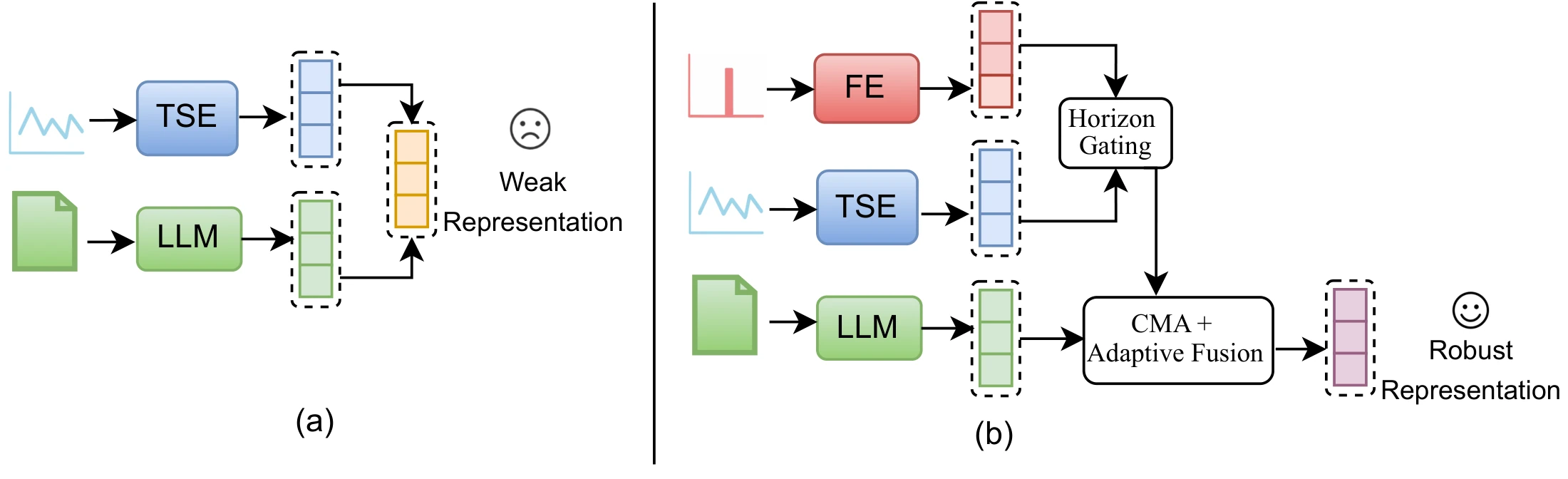
Forecasting models usually commit to one view of the data. Time-domain Transformers such as PatchTST and iTransformer model local dynamics. Frequency models such as FEDformer capture periodicity. LLM-based models such as Time-LLM and TimeCMA describe the series in a text prompt and borrow a language model's priors. Each view sees something the others miss.
- Isolated modalities. Prompt-based models pair time with language but ignore the spectral view that summarizes global periodicity.
- Narrow alignment. A single cross-attention head limits how modalities interact.
- Horizon rigidity. The same fusion is used for every forecast length, although short horizons lean on local detail and long horizons on periodic structure.
Method
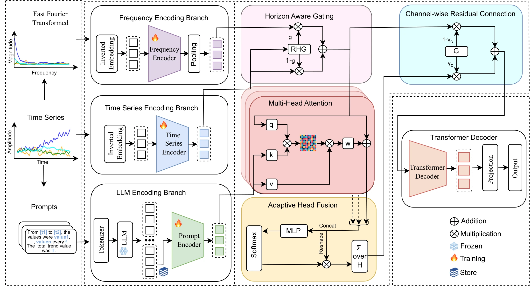
Encode three views, gate by horizon, align, keep a residual path
1. Tri-modal encoding
Frequency. The input is transformed with a real FFT and each magnitude bin becomes a token. After a one-layer Transformer, an attention-weighted pooling summarizes the spectrum per variable.
Time. Each variable's window is linearly embedded and encoded by a Transformer.
Language. Each variable gets a prompt such as "From [t1] to [t2], the values were [v1, …, vn] every [hour]. The total trend value was [T]." A frozen GPT-2 encodes it, and the last-token embedding is kept.
2. Horizon-aware gating
A small MLP reads the pooled time encoding together with the normalized prediction length and outputs per-channel gates. Each forecast horizon gets its own mix of spectral and temporal evidence.
3. Adaptive multi-head cross-modal alignment
Instead of one cross-attention head, \(H\) independent heads align the gated series features (queries) with the prompt embeddings (keys and values). A gating network then scores the heads separately for every variable, so different variables can rely on different alignments.
4. Channel-wise residual fusion
Learned per-channel coefficients decide how much each latent channel takes from the aligned features versus the raw temporal–spectral path, before a Transformer decoder and a linear forecasting head.
Results
Long-term forecasting · averaged over four horizons · lower is better
Following TimeCMA, inputs are 96 steps and horizons are {96, 192, 336, 720} (36 steps and {24, 36, 48, 60} for ILI), averaged over three seeds.
MSE
| Dataset | T3Time | TimeCMA | Time-LLM | UniTime | TimesNet | DLinear | iTransformer | PatchTST | OFA |
|---|---|---|---|---|---|---|---|---|---|
| ETTm1 | 0.372 | 0.380 | 0.410 | 0.385 | 0.400 | 0.403 | 0.407 | 0.392 | 0.396 |
| ETTm2 | 0.279 | 0.275 | 0.296 | 0.293 | 0.291 | 0.350 | 0.288 | 0.285 | 0.294 |
| ETTh1 | 0.418 | 0.423 | 0.448 | 0.442 | 0.458 | 0.456 | 0.454 | 0.463 | 0.457 |
| ETTh2 | 0.348 | 0.372 | 0.381 | 0.378 | 0.414 | 0.559 | 0.383 | 0.395 | 0.389 |
| ECL | 0.170 | 0.174 | 0.195 | 0.216 | 0.192 | 0.212 | 0.178 | 0.207 | 0.217 |
| Weather | 0.244 | 0.250 | 0.275 | 0.253 | 0.259 | 0.265 | 0.258 | 0.257 | 0.279 |
| ILI | 1.705 | 1.922 | 2.432 | 2.108 | 2.139 | 2.616 | 2.444 | 2.388 | 2.623 |
| Exchange | 0.353 | 0.395 | 0.372 | 0.364 | 0.416 | 0.354 | 0.360 | 0.390 | 0.519 |
MAE
| Dataset | T3Time | TimeCMA | Time-LLM | UniTime | TimesNet | DLinear | iTransformer | PatchTST | OFA |
|---|---|---|---|---|---|---|---|---|---|
| ETTm1 | 0.393 | 0.392 | 0.409 | 0.399 | 0.406 | 0.407 | 0.410 | 0.402 | 0.401 |
| ETTm2 | 0.322 | 0.323 | 0.340 | 0.334 | 0.333 | 0.401 | 0.332 | 0.328 | 0.339 |
| ETTh1 | 0.430 | 0.431 | 0.443 | 0.448 | 0.450 | 0.452 | 0.447 | 0.449 | 0.450 |
| ETTh2 | 0.390 | 0.397 | 0.404 | 0.403 | 0.427 | 0.515 | 0.407 | 0.414 | 0.414 |
| ECL | 0.266 | 0.269 | 0.288 | 0.306 | 0.295 | 0.300 | 0.270 | 0.289 | 0.308 |
| Weather | 0.275 | 0.276 | 0.291 | 0.276 | 0.287 | 0.317 | 0.278 | 0.280 | 0.297 |
| ILI | 0.835 | 0.921 | 1.012 | 0.929 | 0.931 | 1.090 | 1.203 | 1.011 | 1.060 |
| Exchange | 0.401 | 0.429 | 0.416 | 0.404 | 0.443 | 0.414 | 0.403 | 0.429 | 0.500 |
Few-shot forecasting
With only a tenth or a twentieth of the training data, T3Time beats the strongest baseline on all five datasets.
| Dataset | T3Time (10%) | Best baseline (10%) | T3Time (5%) | Best baseline (5%) |
|---|---|---|---|---|
| ETTm1 | 0.376 | 0.387 (TimeCMA) | 0.384 | 0.396 (TimeCMA) |
| ETTm2 | 0.266 | 0.277 (Time-LLM) | 0.267 | 0.274 (Time-LLM) |
| ETTh1 | 0.449 | 0.480 (TimeCMA) | 0.442 | 0.472 (TimeCMA) |
| ETTh2 | 0.357 | 0.370 (Time-LLM) | 0.357 | 0.382 (Time-LLM) |
| Weather | 0.226 | 0.229 (TimeCMA) | 0.226 | 0.231 (TimeCMA) |
MSE, lower is better. Average reductions are 3.62% (10%) and 4.13% (5%).
What matters
Ablations · MSE
| Dataset | T3Time | w/o frequency | w/o multi-head CMA | w/o residual | w/o gating |
|---|---|---|---|---|---|
| ETTm1 | 0.372 | 0.381 | 0.374 | 0.404 | 0.373 |
| ETTm2 | 0.279 | 0.279 | 0.283 | 0.288 | 0.280 |
| ETTh1 | 0.418 | 0.433 | 0.421 | 0.433 | 0.425 |
| ETTh2 | 0.348 | 0.364 | 0.355 | 0.384 | 0.363 |
| Weather | 0.244 | 0.250 | 0.249 | 0.249 | 0.249 |
| ILI | 1.705 | 1.786 | 1.813 | 2.176 | 1.724 |
| Exchange | 0.353 | 0.374 | 0.378 | 0.396 | 0.373 |
- The residual path matters most. Without it, MSE rises on every dataset, from 1.705 to 2.176 on ILI.
- The spectral view pays off on periodic data, such as Exchange (0.353 → 0.374) and ILI (1.705 → 1.786).
- Multi-head alignment and horizon gating each give consistent smaller gains.
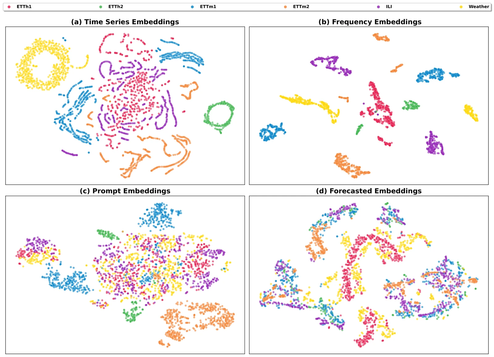
What the three views learn
Limitations
Experiments use standard public benchmarks and a frozen GPT-2 for the language branch. Larger-scale pretraining and richer representations for each modality are left for future work.
Citation
@inproceedings{chowdhury2026t3time,
  title     = {{T3Time}: Tri-Modal Time Series Forecasting via Adaptive
               Multi-Head Alignment and Residual Fusion},
  author    = {Chowdhury, Abdul Monaf and Akter, Rabeya and Arib, Safaeid Hossain},
  booktitle = {Proceedings of the AAAI Conference on Artificial Intelligence},
  volume    = {40},
  number    = {25},
  pages     = {20597--20605},
  year      = {2026},
  doi       = {10.1609/aaai.v40i25.39196}
}